Simulated annealing
Last week I wrote about Evolving Non-Determinism. I briefly mentioned Simulated Annealing. Also someone asked on Reddit about these two
What are the pros and cons of Evolving Nondeterminism vs Simulated Annealing?
One is not strictly better than another. Which one you could use depends on the problem. In this post I will show my results with three problems, ramp and finnish randonneur (travelling salesman) already presented in evolving non-determinism post, and another problem: Generating magic constants for SplitMix16 algorithm (16bit variant of SplitMix).
#Overview of Simulated Annealing
We will begin with a review of the simulated annealing. The problem definition in Haskell terms could look like:
type Probability = Double

data Problem metric beta solution = Problem
    { initial    :: SMGen -> solution
    , neighbor   :: SMGen -> solution -> solution
    , fitness    :: solution -> metric
    , schedule   :: [beta]
    , acceptance :: solution -> solution
                 -> metric -> metric
                 -> beta
                 -> Probability
    }
We use Doubles from 0 to 1 as Probability. And the Problem consists from five fields:
initialsolution. Technically it could be some fixed solution, we don't need to generate it randomly.neighborproduces a random neighbor complete solution from another complete solution. Notice that simulated annealing works only with complete solutions.fitnesstells some metric about the solution. Technically we don't need one, but in practice we probably have one.scheduleis the "annealing schedule". In other words how we "cool down" the random walk in the solution space.acceptancetells the probability of whether we should accept the new solution, given old and new ones, their metrics and current temperature,beta. (betais temperature inverse. So we start close to zero, and then increase thebeta, decrease the temperature).
The Wikipedia article on Simulated Annealing tells that method is inspired by metropolis algorithm used for Ising model in statistical physics. They work very similarly:
- We start with
initialsolution - We generate
neighborsolution - Given the current temperature we probabilistically either accept or reject the new solution..
- Loop
Important point about both Ising model and simulated annealing is Ergodicity of the model. In short, it should be possible to reach any state of the state (or solution) space using neighbor function. (The corresponding requirement for evolving non-determinism is that completeSolution spans the whole solutions space).
The tricky part for simulated annealing is to find good acceptance criteria and corresponding schedule. The idea is to allow more random walk in the beginning, but cool it down so a more local optimum will be found.
This is why I think schedule belongs to Problem. Firstly, the type of "temperature" is problem dependent, and secondly, even if it is glorified Double in most cases, the values are also problem specific.
The usual (I guess, I literally have no idea?) way is to always accept a solution which has better fitness, but only accept worse solutions if temperature + luck tells so. In Ising model simulation the acceptance of new state is as follows:
so I used the same idea. (Here, smaller fitness values are better).
newtype D a = D Double

isingAcceptance
    :: D metric -- ^ H(u)
    -> D metric -- ^ H(v)
    -> D beta   -- ^ inverse temperature, \( \beta \).
    -> Probability
isingAcceptance (D hu) (D hv) (D beta)
    | di > 0    = exp (negate (beta * di))
    | otherwise = 1
  where
    di = hv - hu
With three problems we will see, I found it tricky to find these parameters. The upside is that algorithm is quick. I rerun it multiple times with different initial seeds to get another result.
The Evolving Determinism required less "thinking". You can think about disorder thresholds, but most likely you'll get good result anyway (you might spend more time).
#Ramp
The ramp problem is to "sort" the bag of numbers so there are no downhills. One natural choice for neighbor is to pick one index from the list and swap the element with one next to it. This makes system ergodic, as we can get any permutation with just neighbor swaps.
[...3,5,4,6,...]
[...3,4,5,6,...]
The resulting algorithm is not much an improvement over bogosort. In fact, if we are unlucky in the start, having the configuration like:
[9,0,1,2,4,5,6,7,8]it would require a lot of boiling, before 9 moves closer to the end.
The next try is to improve neighbor to pick two indices at once, and swap their elements. Then you would think, that given enough time it will work. It doesn't
I run a ramp problem of 10 elements for 100000 steps 1000 times. So that a the beginning the probability of "unsorting" the solution is 30%, and 0% a the very end. I got optimal result 0 down ramps in 692, and second best with 1 in remaining 308 cases. For bigger problem of 20 elements i run it for 400000 steps 1000 times, and got
0 down ramps:   0 cases
1 down ramps:  70 cases
2 down ramps: 920 cases
3 down ramps:  16 cases
Random sorting is difficult!
In comparison, END found the optimal solution every time, but it took longer to do it. It wasn't randomly sorting, it was randomly picking the smallest element.
#SplitMix16
SplitMix is random number generator. See Guy L. Steele, Jr., Doug Lea, and Christine H. Flood. 2014. Fast splittable pseudorandom number generators. for all the details. We are interested in a mixing functions used in its implementation. In Haskell they look like
mix64 :: Word64 -> Word64
mix64 z0 = let z1 = shiftXorMultiply 33 0xff51afd7ed558ccd z0
               z2 = shiftXorMultiply 33 0xc4ceb9fe1a85ec53 z1
               z3 = shiftXor 33 z2
           in z3

shiftXor :: Int -> Word64 -> Word64
shiftXor n w = w `xor` (w `shiftR` n)

shiftXorMultiply :: Int -> Word64 -> Word64 -> Word64
shiftXorMultiply n k w = shiftXor n w `mult` k
This is a mixer from MurMurHash3, but note the magic constants: three for shift operations (all 33) and two for multiplication (0xff51afd7ed558ccd and 0xc4ceb9fe1a85ec53).
In MurMurHash3 this mixer (or finalizer) is used to obtain better distribution of hashes.
Ideally, flipping a single bit in the input key results in all output bits changing with a probability of 0.5. This is called the Avalanche effect. Our today's task would be to find a good constants for Word16 variant. There we can calculate the strict avalanche criterion exhaustively:
- For all 65536
Word16numbers - For all 16 bits
- Flip a bit, and observe how much bits in output change
In Haskell that looks (behold, mutable vectors ahead):
avalancheStep
    :: Word16
    -> (Word16 -> Word16)
    -> MUV.MVector s Word32
    -> ST s ()
avalancheStep u f vec = do
    for_ [0 .. 15 :: Int] $ \i -> do
        -- with a single bit flipped
        let v = complementBit u i

        -- apply function
        let u' = f u
            v' = f v

        -- for each output bit
        for_ [0 .. 15 :: Int] $ \j -> do
            let ne = u' `xor` v'

            -- check when they are not the same
            when (testBit ne j) $ MUV.unsafeModify vec succ (i * 16 + j)
At the end we get 256 numbers, which all should be roughly the same close to 32768.
If you read the Steele's paper closely, you may notice an error in SplitMix code figure but there's also an error in avalanche metric algorithm they show (Figure 18 in http://gee.cs.oswego.edu/dl/papers/oopsla14.pdf version).
Here's some C code. Based on the text of the paper author used something like the second variant. Yet the code in the paper seems to center the distribution (double v = a[j][k] - N / 2.0). Another hint that it's not "real" code is that there's both mix64 and m.mix used to call mixing function. Anyway, luckily for us, paper has enough "redundancy", as there is prose explaining what code of figures tries to do. (Commenting your non-trivial code is important: when code and comments disagree, you at least have a hint that either is wrong!)
#include <stdio.h>
#include <stdint.h>

/* murmurhash 32 mixer */
uint32_t mix(uint32_t h) {
    h ^= h >> 16;
    h *= 0x85ebca6b;
    h ^= h >> 13;
    h *= 0xc2b2ae35;
    h ^= h >> 16;
    return h;
}

#define N  100000
#define HN  50000.0L

/*  https://dl.acm.org/doi/pdf/10.1145/2660193.2660195?download=true */

int main() {
    long A [64][64];

    for (uint32_t n = 0; n < N; n++) {
        uint32_t v = n;
        uint32_t w = mix(v);

        for (int i = 0; i < 32; i++) {
            uint32_t x = w ^ mix(v ^ (1 << i));
            for (int j = 0; j < 32; j++) {
                if (((x >> j) & 1) != 0) {
                    A[i][j] += 1;
                }
            }
        }
    }

    /* this centers the distribution before taking square,
       so "best" is 0 */
    {
        double sumsq = 0.0;
        for (int i = 0; i < 32; i++) {
            for (int j = 0; j < 32; j++) {
                double v = (A[i][j] - HN) / HN;
                printf("%+.3lf ", 10 * v);
                sumsq += v*v;
            }
            printf("\n");
        }

        double result = sumsq / (32 * 32);

        printf("result %lf\n", result);
    }

    /* this doesn't center the distribution,
       so "best" is 1 */
    {
        double sumsq = 0.0;
        for (int i = 0; i < 32; i++) {
            for (int j = 0; j < 32; j++) {
                double v = A[i][j] / HN;
                sumsq += v*v;
            }
        }

        double result = sumsq / (32 * 32);

        printf("result %lf\n", result);
    }
}
I chose to use the first variant, because then the fitness metric is simple: the smaller the better. We can "test" that the metric works:
*SA SA.Example.SplitMix16> avalanche id
1.000000
(12.03 secs, 10,881,343,744 bytes)

*SA SA.Example.SplitMix16> avalanche exampleHash
0.006548
(19.29 secs, 15,551,170,904 bytes)

*SA SA.Example.SplitMix16> avalanche truncated16MD5
0.000032
(20.75 secs, 16,345,429,696 bytes)
Notice that evaluating avalanche takes some time, less when compiled than in GHCi but some time. Let us say, a second when compiled.
The identity function is very bad mixer (the 1.0 is about as bad as it can be). The exampleHash (with just some constants) is performing clearly better. [MD5] (which is cryptographic, though weak hash function) avalance value is two magnitudes better; but it's also slower (note that exampleHash is interpreted, and MD5 is running optimized version. Still exampleHash is faster) With this avalanche metric in place we can look for good parameters for our mix16 variant. Here I already fixed the shift constants.
paramHash
    :: Word16   -- ^ param1
    -> Word16   -- ^ param2
    -> Word16   -- ^ input
    -> Word16   -- ^ output
paramHash p0 p1 x0 =
    let x1 = x0 `xor` (x0 `shiftR` 8)
        x2 = x1 * p0
        x3 = x2 `xor` (x1 `shiftR` 5)
        x4 = x3 * p1
        x5 = x4 `xor` (x4 `shiftR` 8)
    in x5
We cannot test the whole search space (2^32 options) exhaustively, but we can use simulated annealing. Params are self-explanatory:
data Params = Params !Word16 !Word16The fitness function is not surprising either:
fitness (Params p0 p1) = avalanche (paramHash p0 p1)Also all Params are valid solutions, so picking neighbor is easy. It seems that flipping one bit in Params doesn't cause massive changes in avalanche so it works.
neighbor g (Params p0 p1) =
    -- there are 32 possible bits we can flip
    let i = fromIntegral $ fst $ SM.bitmaskWithRejection64 32 g
    in if i < 16
       then Params (complementBit p0 i) p1
       else Params p0 (complementBit p1 (i - 16))
After some runs (each of which takes about 3 minutes on a single core) I found some possible parameters:
Params 0xd255 0xed45; avalanche = 0.000366
Params 0x8595 0xeebb; avalanche = 0.000390
Params 0xf7d5 0x314b; avalanche = 0.000436
We got closer to MD5's avalanche value, but are still far. Therefore, when I did similar optimization for SplitMix32 constants, I run statistical tests on the resulting random number generator. SplitMix32 passes dieharder test suite, for example.
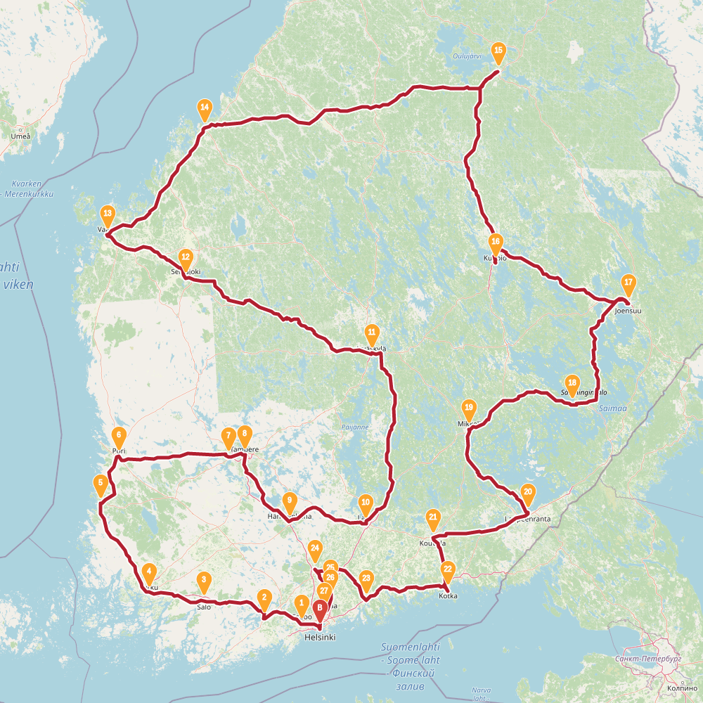
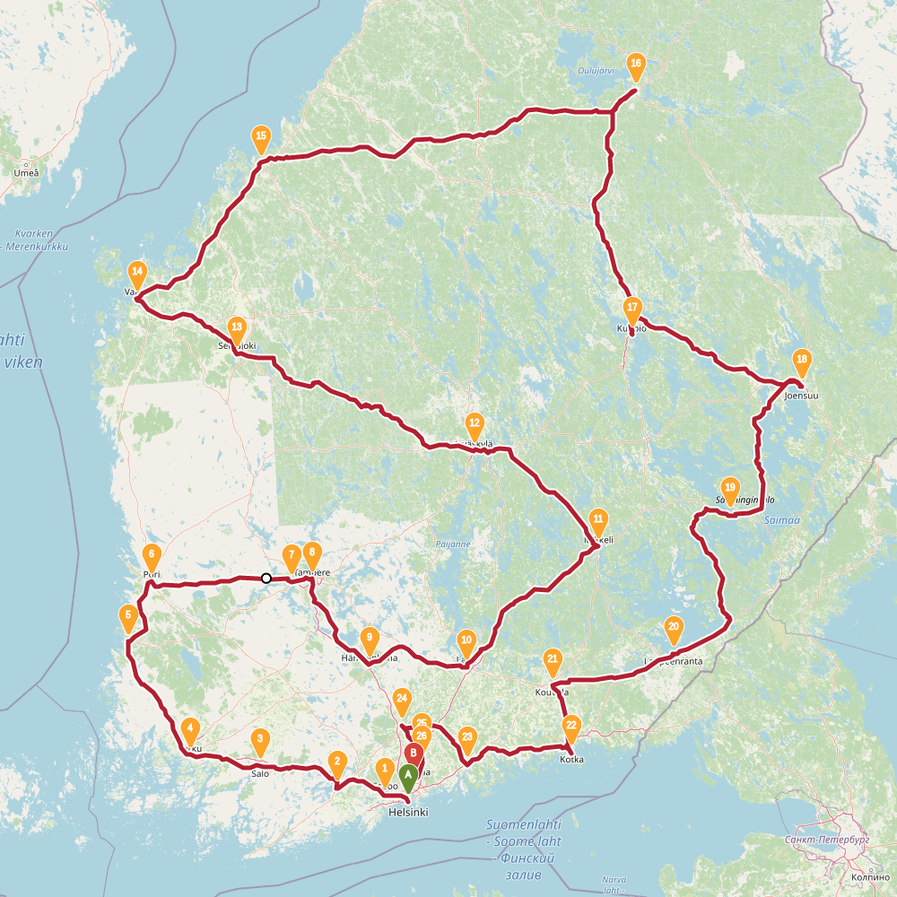
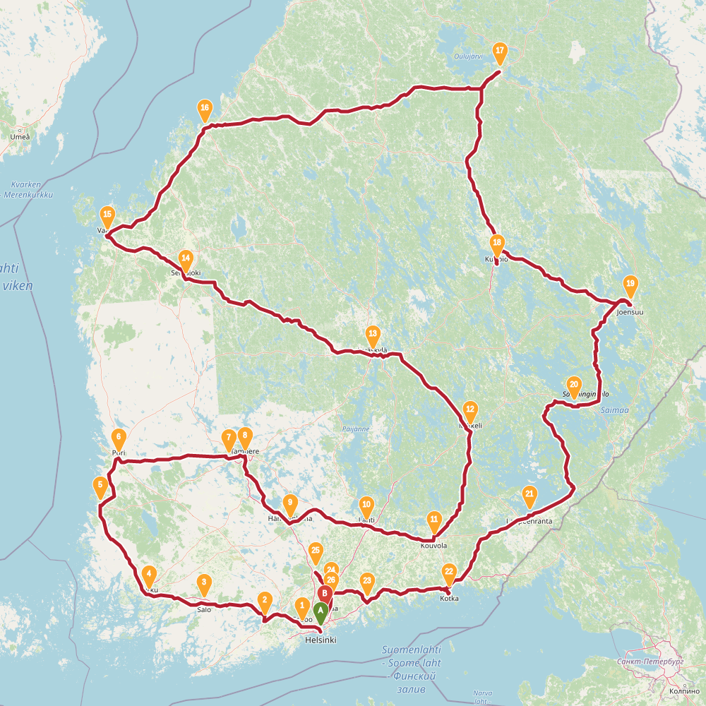
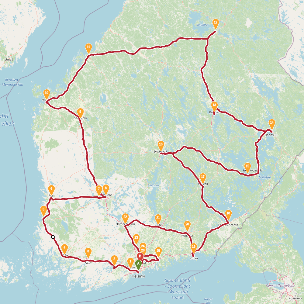
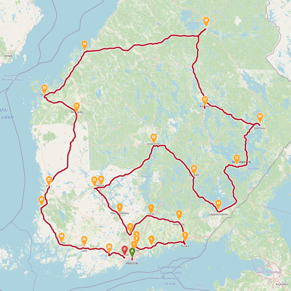
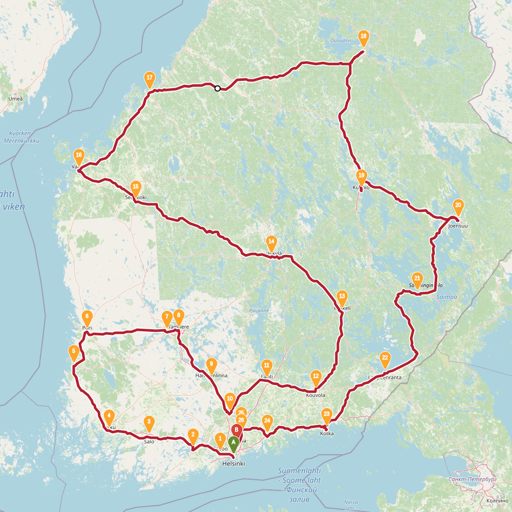
#Finnish Randonneur
Finnish randonneur is a traveling salesman problem. The task is to find a route through 30 biggest cities of Finland.
In this problem the simulated annealing performed relatively well. In the table below is summary of results. The left column is results found with evolving non-determinism, the right column is 4 new results found with simulated annealing.
SA found two results shorter than previously known. However typical run resulted in a route over 2500km. The new shorter solutions are quite different around Helsinki, the starting point used for END. This highlights the problem with evolving non-determinism: the choices we made around start and end globally affected the results. Recall that we build up solution into both directions simultaneously. Maybe our overall population was too small, or disorder threshold too low. Impossible to tell now.
Changing the initial city to Oulu (i.e. something in the north) gave a solution with 2435 distance on the first rerun of END algorithm. But it still wasn't able to find the 2422 solution in a dozen more runs.
The topology of the solution space for this problem is much more interesting than I thought.
 2447 |
 2422 |
 2449 |
 2470 |
 2461 |
 2441 |
 2451 |
#Conclusion
I presented simulated annealing on three different problems, two of which are the same as I used with evolving non-determism
| Problem | END | SA |
|---|---|---|
| Ramp | perfect results | good results, quicker |
| Finnish Randonneur (TSP) | good results | more variance, quicker |
| SplitMix | bad fit | good |
| Sorting Networks | good | bad fit |
With ramp problem END performed perfectly, which is not surprising, as it is a problem ``designed'' to make all other methods look worse in comparison.
With TSP both END and SA performed well, with a human in the loop using SA results we have been able to improve END results. With this problem, I have to find better way to model it for END, so it wouldn't stuck in local optima (which was good though).
The SplitMix problem presented in this blog post is well suited for SA. I tried END on it too, but it's bad. My idea was to pick up to five bits to flip. Whether that makes sense in the solution space topology is unknown, and what is the suitable "prefix". It didn't work out.
Correspondingly, I didn't even try to apply SA for sorting network problem. What would be a good neighbor function?
It's good to look at SplitMix and sorting network problem properties:
| SplitMix | Sorting networks | TSP | |
|---|---|---|---|
| Ergodicity | easy | tricky | moderate |
| Fitness function | slow | quick | quick |
| Constructing solutions | quick | slow | quick |
| Solution | is unordered | is ordered | has some ordering |
Evaluating fitness function of SplitMix is slow, and for sorting networks constructing a solution in first place is slow process. I think this differentiates them. On the other hand, TSP is "easy" problem so either method perform well enough.
Finally, I want to highlight maybe not so obvious thing from this and previous post: Haskell language is a good fit for both modeling of computational methods and actually running them on "normal sized" (i.e. not "toy sized") problems. A very nice property for a programming language.
- 2026-05-07 – Compatibility packages in 2026
- 2025-02-13 – PHOAS to de Bruijn conversion
- 2025-02-11 – NbE PHOAS
- 2024-06-24 – hashable arch native
- 2024-05-28 – cabal fields
 This work is licensed under a “CC BY SA 4.0” license.